

The Test System: Corn Cobs
On a cob of corn, each kernel has resulted from an independent fertilization event. Each kernel therefore is like one child, and each cob is like a family of siblings, all with the same parents. By observing a group of kernels on the same cob, you can observe a single generation of offspring resulting from a single cross. This is why corn cobs are a useful way to study Mendelian ratios in genetics.
Colour (purple or yellow) and texture (smooth or wrinkled) of corn kernels can each be associated with single genes. Assume that each of these traits has two alleles, one dominant and one recessive. In this lab, you will be coming up with hypotheses about the inheritance of these traits in corn. You will then use your hypothesis to generate a prediction about the outcome of an experimental genetic cross. To move from your hypothesis to an experimentally testable prediction, you will make use of Punnett squares, just as you did in the warm-up exercises. The resulting offspring (corn kernels) from these genetic crosses are pictured on the following pages. You will observe the phenotypes of these offspring to see how well the actual, observed results match with the results predicted by your hypothesis. (Remember that you cannot directly observe genotype, only phenotype!) If the observed results do not match the predicted results closely enough, you will reject your hypothesis. If the observed results do match the predicted results closely enough, then you will not reject your hypothesis.
But how close is "close enough"? Even if your hypothesis is a good one, the observed and predicted numbers of kernels of a particular phenotype will probably not match exactly: there will be a bit of variation due to chance. In this lab, you will do a statistical test called the chi-squared test of goodness of fit. This is a mathematical way of saying whether or not your observed and expected results match closely enough for you to hang on to your hypothesis (that is, to "not reject" it - in statistics we never support or verify a hypothesis, we merely fail to reject it).
At the end of your chi-squared test, you will end up with a p-value: this is a value that tells you how likely it is that the difference between what you observed and what you expected is due to chance alone (rather than being due to your hypothesis being wrong!). If your p-value is large, then you do not reject your hypothesis: for example, a p-value of 0.5 tells you that there is a 50% probability that the difference between observed and expected results was due to chance - so you won't reject that hypothesis. If your p-value is small (less than 0.05, which means less than a 5% chance that the difference between observed and expected results was due to chance), then you will reject your hypothesis. The differences between what you observed and what you expected to observe were probably due to an incorrect hypothesis, rather than to chance alone.
A Useful Tool: ImageJ
You used the ImageJ in the Cells and Diffusion lab to measure diameters of red blood cells, and you will need it again in this lab to count corn kernels of different types (yellow, purple, smooth, wrinkled, etc.). This time you will have to download and install the entire ImageJ program, as the Cell Counter function that you will be using is not available on the applet. Download and installation, however, is fast and easy:
1. Start by going to http://imagej.nih.gov/ij/ to download the program.
2. Download the ImageJ package and extract the ImageJ directory as instructed.
3. Start the program; a small ImageJ dialog box will appear on your screen (upper right in the screen cap below).
4. Return to this lab and right-click on the corn cob photos (on the following pages) to save copies of the images. Use ImageJ (File --> Open...) to open the photo that you want to count kernels on.
5. From the ImageJ Plugins drop-down menu, go to Analyze --> Cell Counter. The Cell Counter dialog box will appear. Click on the Initialize button. (If you don't, you'll be prompted to do so.)
6. Choose the Type 1 counter, then move your mouse over to the corn photo and start clicking on the individual kernel types you want to count. You just have to click on kernels; the Cell Counter will keep a running tally in the box adjacent to 'Type 1'. When you're finished clicking on 5 rows' worth of kernels, note the total in the Cell Counter.
7. Switch to the Type 2 counter and count up the next type of kernels. Note the total in the Cell Counter dialog box.
8. Continue as necessary until you have counted all of the different types of kernels you need to.
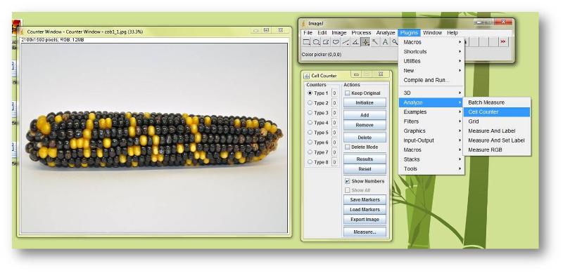
Image Credits
ImageJ screen capture by Jennifer Van Dommelen